word2vec

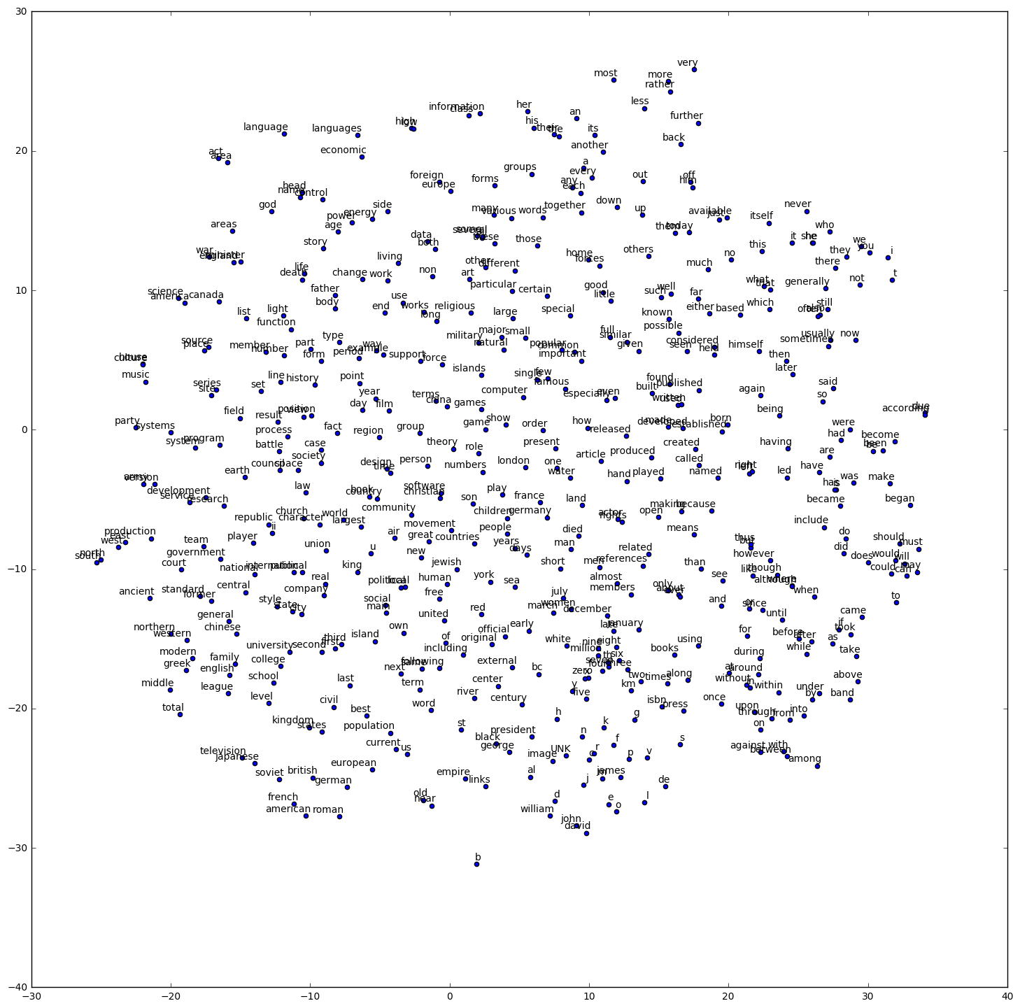
word2vec는 비슷한 단어들끼리 집단화(clustering)시키는 모델입니다. 실습을 위한 아래 코드는 TensorFlow tutorial word2vec의 내용입니다. 이를 참고해서 word2vec를 학습하도록 합시다. 또한 관련 문서는 텐서플로우 문서 한글 번역본을 참고하도록 합니다.

# Copyright 2015 The TensorFlow Authors. All Rights Reserved.
#
# Licensed under the Apache License, Version 2.0 (the "License");
# you may not use this file except in compliance with the License.
# You may obtain a copy of the License at
#
#     http://www.apache.org/licenses/LICENSE-2.0
#
# Unless required by applicable law or agreed to in writing, software
# distributed under the License is distributed on an "AS IS" BASIS,
# WITHOUT WARRANTIES OR CONDITIONS OF ANY KIND, either express or implied.
# See the License for the specific language governing permissions and
# limitations under the License.
# ==============================================================================

from __future__ import absolute_import
from __future__ import division
from __future__ import print_function

import collections
import math
import os
import random
import zipfile

import numpy as np
from six.moves import urllib
from six.moves import xrange  # pylint: disable=redefined-builtin
import tensorflow as tf

# Step 1: 데이터를 다운로드 합니다.
url = 'http://mattmahoney.net/dc/'

def maybe_download(filename, expected_bytes):
  """Download a file if not present, and make sure it's the right size."""
  if not os.path.exists(filename):
    filename, _ = urllib.request.urlretrieve(url + filename, filename)
  statinfo = os.stat(filename)
  if statinfo.st_size == expected_bytes:
    print('Found and verified', filename)
  else:
    print(statinfo.st_size)
    raise Exception(
        'Failed to verify ' + filename + '. Can you get to it with a browser?')
  return filename

filename = maybe_download('text8.zip', 31344016)


# 데이터를 읽어서 리스트에 문자열을 넣습니다.
def read_data(filename):
  """Extract the first file enclosed in a zip file as a list of words"""
  with zipfile.ZipFile(filename) as f:
    data = tf.compat.as_str(f.read(f.namelist()[0])).split()
  return data

words = read_data(filename)
print('Data size', len(words))

# Step 2: 사전을 구축하고 드문 단어를 UNK 토큰으로 변경합니다.
vocabulary_size = 50000

def build_dataset(words):
  count = [['UNK', -1]]
  count.extend(collections.Counter(words).most_common(vocabulary_size - 1))
  dictionary = dict()
  for word, _ in count:
    dictionary[word] = len(dictionary)
  data = list()
  unk_count = 0
  for word in words:
    if word in dictionary:
      index = dictionary[word]
    else:
      index = 0  # dictionary['UNK']
      unk_count += 1
    data.append(index)
  count[0][1] = unk_count
  reverse_dictionary = dict(zip(dictionary.values(), dictionary.keys()))
  return data, count, dictionary, reverse_dictionary

data, count, dictionary, reverse_dictionary = build_dataset(words)
del words  # Hint to reduce memory.
print('Most common words (+UNK)', count[:5])
print('Sample data', data[:10], [reverse_dictionary[i] for i in data[:10]])

data_index = 0

# Step 3: skip-gram 모델에 대한 훈련 배치를 생성하는 함수.
def generate_batch(batch_size, num_skips, skip_window):
  global data_index
  assert batch_size % num_skips == 0
  assert num_skips <= 2 * skip_window
  batch = np.ndarray(shape=(batch_size), dtype=np.int32)
  labels = np.ndarray(shape=(batch_size, 1), dtype=np.int32)
  span = 2 * skip_window + 1  # [ skip_window target skip_window ]
  buffer = collections.deque(maxlen=span)
  for _ in range(span):
    buffer.append(data[data_index])
    data_index = (data_index + 1) % len(data)
  for i in range(batch_size // num_skips):
    target = skip_window  # target label at the center of the buffer
    targets_to_avoid = [skip_window]
    for j in range(num_skips):
      while target in targets_to_avoid:
        target = random.randint(0, span - 1)
      targets_to_avoid.append(target)
      batch[i * num_skips + j] = buffer[skip_window]
      labels[i * num_skips + j, 0] = buffer[target]
    buffer.append(data[data_index])
    data_index = (data_index + 1) % len(data)
  return batch, labels

batch, labels = generate_batch(batch_size=8, num_skips=2, skip_window=1)
for i in range(8):
  print(batch[i], reverse_dictionary[batch[i]],
        '->', labels[i, 0], reverse_dictionary[labels[i, 0]])

# Step 4: skip-gram 모델을 구축하고 훈련하십시오.

batch_size = 128
embedding_size = 128  # Dimension of the embedding vector.
skip_window = 1       # How many words to consider left and right.
num_skips = 2         # How many times to reuse an input to generate a label.

# We pick a random validation set to sample nearest neighbors. Here we limit the
# validation samples to the words that have a low numeric ID, which by
# construction are also the most frequent.
valid_size = 16     # Random set of words to evaluate similarity on.
valid_window = 100  # Only pick dev samples in the head of the distribution.
valid_examples = np.random.choice(valid_window, valid_size, replace=False)
num_sampled = 64    # Number of negative examples to sample.

graph = tf.Graph()

with graph.as_default():

  # Input data.
  train_inputs = tf.placeholder(tf.int32, shape=[batch_size])
  train_labels = tf.placeholder(tf.int32, shape=[batch_size, 1])
  valid_dataset = tf.constant(valid_examples, dtype=tf.int32)

  # Ops and variables pinned to the CPU because of missing GPU implementation
  with tf.device('/cpu:0'):
    # Look up embeddings for inputs.
    embeddings = tf.Variable(
        tf.random_uniform([vocabulary_size, embedding_size], -1.0, 1.0))
    embed = tf.nn.embedding_lookup(embeddings, train_inputs)

    # Construct the variables for the NCE loss
    nce_weights = tf.Variable(
        tf.truncated_normal([vocabulary_size, embedding_size],
                            stddev=1.0 / math.sqrt(embedding_size)))
    nce_biases = tf.Variable(tf.zeros([vocabulary_size]))

  # Compute the average NCE loss for the batch.
  # tf.nce_loss automatically draws a new sample of the negative labels each
  # time we evaluate the loss.
  loss = tf.reduce_mean(
      tf.nn.nce_loss(nce_weights, nce_biases, embed, train_labels,
                     num_sampled, vocabulary_size))

  # Construct the SGD optimizer using a learning rate of 1.0.
  optimizer = tf.train.GradientDescentOptimizer(1.0).minimize(loss)

  # Compute the cosine similarity between minibatch examples and all embeddings.
  norm = tf.sqrt(tf.reduce_sum(tf.square(embeddings), 1, keep_dims=True))
  normalized_embeddings = embeddings / norm
  valid_embeddings = tf.nn.embedding_lookup(
      normalized_embeddings, valid_dataset)
  similarity = tf.matmul(
      valid_embeddings, normalized_embeddings, transpose_b=True)

  # Add variable initializer.
  #init = tf.global_variables_initializer()
  init = tf.initialize_all_variables()

# Step 5: 훈련을 시작하십시오.
num_steps = 100001

with tf.Session(graph=graph) as session:
  # We must initialize all variables before we use them.
  init.run()
  print("Initialized")

  average_loss = 0
  for step in xrange(num_steps):
    batch_inputs, batch_labels = generate_batch(
        batch_size, num_skips, skip_window)
    feed_dict = {train_inputs: batch_inputs, train_labels: batch_labels}

    # We perform one update step by evaluating the optimizer op (including it
    # in the list of returned values for session.run()
    _, loss_val = session.run([optimizer, loss], feed_dict=feed_dict)
    average_loss += loss_val

    if step % 2000 == 0:
      if step > 0:
        average_loss /= 2000
      # The average loss is an estimate of the loss over the last 2000 batches.
      print("Average loss at step ", step, ": ", average_loss)
      average_loss = 0

    # Note that this is expensive (~20% slowdown if computed every 500 steps)
    if step % 10000 == 0:
      sim = similarity.eval()
      for i in xrange(valid_size):
        valid_word = reverse_dictionary[valid_examples[i]]
        top_k = 8  # number of nearest neighbors
        nearest = (-sim[i, :]).argsort()[1:top_k + 1]
        log_str = "Nearest to %s:" % valid_word
        for k in xrange(top_k):
          close_word = reverse_dictionary[nearest[k]]
          log_str = "%s %s," % (log_str, close_word)
        print(log_str)
  final_embeddings = normalized_embeddings.eval()

# Step 6: 임베딩을 시각화합니다.

def plot_with_labels(low_dim_embs, labels, filename='tsne.png'):
  assert low_dim_embs.shape[0] >= len(labels), "More labels than embeddings"
  plt.figure(figsize=(18, 18))  # in inches
  for i, label in enumerate(labels):
    x, y = low_dim_embs[i, :]
    plt.scatter(x, y)
    plt.annotate(label,
                 xy=(x, y),
                 xytext=(5, 2),
                 textcoords='offset points',
                 ha='right',
                 va='bottom')

  plt.savefig(filename)
  #plt.show()

try:
  # jupyter notebook을 위한 코드입니다.
  # pycharm 등에서 실행하려면 plot_with_labels()함수에 plt.show()를 주석 해제하십시오.
  %pylab inline

  from sklearn.manifold import TSNE
  import matplotlib.pyplot as plt
  # 한글의 경우 plt 그래프에서 깨지므로 아래 주석을 해제하고 폰트를 지정해서 사용하십시오.
  """
  from matplotlib import font_manager, rc

  font_name = font_manager.FontProperties(fname="/usr/share/fonts/truetype/nanum/NanumGothic.ttf").get_name()
  rc('font', family=font_name)
  """

  tsne = TSNE(perplexity=30, n_components=2, init='pca', n_iter=5000)
  plot_only = 500
  low_dim_embs = tsne.fit_transform(final_embeddings[:plot_only, :])
  labels = [reverse_dictionary[i] for i in xrange(plot_only)]
  plot_with_labels(low_dim_embs, labels)

except ImportError:
  print("Please install sklearn, matplotlib, and scipy to visualize embeddings.")

global_variables_initializer() 함수는 0.12 버전부터 제공됩니다. 그 이하 버전에서실습 할 때는 initialize_all_variables() 함수를 사용하도록 합니다.

jupyter notebook으로 실습할 때 그래프가 시각화되지 않는 문제가 있는데 중간에 %pylab inline을 사용해서 문제를 해결 할 수 있습니다. % pylab은 ipython에 magic function입니다. 더 자세한 내용은 이곳에서 참고할 수 있습니다.